Joe Archondis
July 7, 2026 · 12 min read
Fintech & Algo Trading
Backtesting Infrastructure Design: How to Build It Right
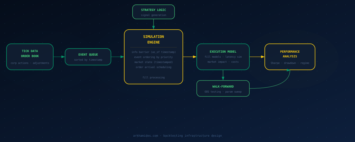
At Enigma Securities, I ran the same mean reversion strategy through two backtesting implementations. One produced a 1.8 Sharpe ratio. The other produced 0.4. Same signal logic. Same historical data. The difference: how each engine simulated the latency between signal generation and order arrival at the exchange. That 1.4-point Sharpe gap was entirely fictitious profit. It disappears the moment you go live.
Building a backtester that produces numbers is a weekend project. Building one you can actually trade against requires a different level of infrastructure rigor. This is what that looks like.
Why Most Backtests Lie
The failure mode isn't usually a bug. It's a collection of optimistic assumptions that each seem reasonable individually but stack into something damaging.
You assume orders fill at the quoted price. You assume zero market impact. You run parameter optimization and performance evaluation on the same dataset. You don't simulate the 8-12ms of latency between signal firing and order arrival at the exchange. Each assumption adds a sliver of fictitious alpha. They compound.
In HFT, latency assumptions alone can swing annual performance by hundreds of basis points. A mean reversion strategy operating on a 1ms price edge looks completely different at 8ms of simulated execution latency. If the backtester doesn't model that gap, it's measuring an imaginary strategy.
Three structural problems to eliminate before anything else:
- Look-ahead bias: using information that wasn't available at the moment of the decision
- Execution optimism: assuming fills that wouldn't happen in practice
- Overfitting: selecting parameters on the same data used for evaluation
None of these are fixable in post-processing. They require structural decisions in how the backtester is built from the start.
The Data Layer
Data is where backtesting infrastructure fails most silently. Not usually because of access problems. Because of granularity, correctness, and the assumptions baked into how data is stored.
Tick data versus bar data: bar data (OHLCV candles) works for swing strategies with multi-day holding periods. For anything operating intraday, you need tick-level data — every trade print and quote update. Bar data destroys the intraday price path and makes realistic execution modeling impossible. You end up simulating fills against close prices that didn't exist when your strategy signal fired.
Order book depth: if your strategy is sensitive to spread or queue position, top-of-book data isn't enough. You need full order book snapshots — L2 (ten price levels each side) at minimum for market-making or aggressive liquidity-taking strategies. Storing L2 data efficiently matters. An uncompressed feed generates several gigabytes per day per instrument.
Corporate actions are one of the quieter ways to corrupt an equity backtest. Dividend and split adjustments need to be applied correctly, with the right direction for your use case: forward-adjusted prices for display, backward-adjusted prices for return calculations. Mixing these up silently breaks P&L arithmetic over multi-year periods.
Your data layer also needs to distinguish between a genuine period of no trading and a feed connectivity gap. Thirty minutes of silence during a major news event should trigger different strategy behavior than thirty minutes caused by a failed reconnection. Build explicit gap metadata alongside your price data.
Storage format decisions matter at scale. At Enigma, we stored tick data in a custom binary format: a fixed header with instrument metadata, then fixed-width 40-byte records — nanosecond timestamp, price, size, side, and flags. Memory-mapped reads, zero parsing overhead on replay. For batch processing, Parquet with snappy compression is the practical choice.
| Format | Best For | Compression | Query Speed |
|---|---|---|---|
| Custom binary (mmap) | Tick-speed replay | Best | Fastest |
| Parquet (snappy) | Batch processing | Good | Fast (columnar reads) |
| TimescaleDB | Time-series queries | Good | Fast (indexed) |
| CSV | Debug / inspection | None | Slow |
Building the Simulation Engine
The simulation engine replays historical market events and determines exactly what your strategy would have done. One design constraint governs everything else: the strategy can only see information that existed at the current event's timestamp.
The event loop is the foundation:
while events remain:
    event = next_event(queue)           # sorted by timestamp; ties broken by type priority
    update_market_state(event)
    if event triggers strategy signal:
        orders = strategy.on_event(event, market_state)
        for order in orders:
            schedule_order_arrival(order, current_time + latency_model())
    process_pending_arrivals()
    process_fills()
Enforce the information barrier explicitly. Your market state object should accept an as_of timestamp and reject any query for data past it. No convenience shortcuts. Every look-ahead bias bug I've encountered came from code reaching into "recent" data without checking the timestamp. It's always subtle. It always inflates results.
Event ordering matters when multiple events share a timestamp, which is common in tick data. Market events first. Strategy decisions second. Order submissions third. Build a priority queue that handles ties in a deterministic, documented order. Undocumented tie-breaking is a bug waiting to surface under unusual market conditions.
Latency scheduling belongs in the event loop, not the strategy. When a strategy fires a signal, the engine schedules order arrival at current_time + latency_sample(). The latency model samples from a distribution parameterized by your real production measurements. Orders arriving in the future then compete against subsequent market events — which is exactly what happens in live trading.
The Execution Model
This is where most backtesting infrastructure fails. The difference between a backtest you can trust and one that flatters you is almost entirely in the execution model.
Latency: model the full round-trip from signal to fill acknowledgment. Strategy computation time, plus network latency to the venue, plus exchange processing time, plus the acknowledgment back. At Enigma, our tick-to-order path ran at 8-12ms in production. Any model assuming sub-millisecond fills was generating results for a strategy that didn't exist. Parameterize your latency distribution from actual production measurements, not vendor spec sheets or theoretical minimums.
Fill models: the naive model — every limit order fills at the quoted price for the full requested size — fails in important ways. Real markets have queue depth ahead of your order. Orders large relative to quoted depth create price impact before fully filling. Partial fills near market close are common. A simple but meaningful model:
def estimate_fill_probability(order_size, depth_at_price):
    if order_size > depth_at_price * 0.5:
        return 0.3    # large relative to depth
    elif order_size > depth_at_price * 0.1:
        return 0.7
    else:
        return 0.95   # small relative to depth, likely fills

def estimate_market_impact(order_size, adv, daily_vol=0.01):
    # Square root law: impact proportional to sqrt of participation rate
    return daily_vol * (order_size / adv) ** 0.5
These are uncalibrated. They're still far more honest than the zero-impact assumption. Calibrate against actual fills once you have production execution data.
Transaction costs: model commissions, exchange fees, and clearing fees from day one — not as a final sensitivity check. For institutional strategies, all-in costs typically run 0.5-2bps per side. A strategy making 5bps average daily is entirely destroyed by 2bps all-in costs. Calculate the breakeven explicitly and include it in every single run from the start.
Out-of-Sample Testing and Walk-Forward Analysis
In-sample performance is a test your strategy always passes. The number that matters is out-of-sample performance on data the strategy never touched during development.
The test set is sacred. Pick it before development begins. Look at it once, after all development is complete. If you peek at out-of-sample results and adjust the model, you've turned it into an in-sample test. The discipline here matters more than any technical sophistication in the rest of your infrastructure.
Walk-forward analysis is more rigorous than a single train/test split. Train on a rolling window, evaluate on the subsequent period, repeat:
Train: 2019-01 to 2021-12  |  Test: 2022 Q1
Train: 2019-04 to 2022-03  |  Test: 2022 Q2
Train: 2019-07 to 2022-06  |  Test: 2022 Q3
...continue forward...
Aggregate performance across all test windows. A strategy showing 1.4 Sharpe in-sample and 0.3 out-of-sample across multiple windows is overfit. One showing 1.1 in-sample and 0.9 out-of-sample consistently is probably real.
Parameter sensitivity testing goes alongside this. Sweep any parameter over a meaningful range and plot performance against it. A robust strategy shows a smooth hill — good results across many values near your chosen one. A sharp peak that degrades quickly on either side is overfitting, not signal.
Performance Analysis That Actually Informs Decisions
Sharpe ratio and maximum drawdown are table stakes. The numbers that tell you whether you've found something real:
Sharpe by regime: does performance hold across different volatility environments? A strategy producing 1.5 Sharpe in low-VIX conditions and destroying capital in high-VIX is a regime bet, not a general alpha source. Segment your results by VIX quartile or realized volatility quartile and compare explicitly. If you only see the aggregate, you won't see this.
Turnover and capacity: high turnover means high costs. A strategy with 400% annual turnover needs roughly 8bps daily gross alpha to survive 2bps all-in transaction costs. Calculate the breakeven. Model how performance degrades as notional size grows. Most alpha strategies have hard capacity limits where fill impact at $10M looks nothing like $1M.
Drawdown duration, not just depth: a 15% drawdown recovering in three weeks is a different kind of risk than one taking 18 months to recover. Both are 15%. They're not the same. Your performance report should show both the magnitude and the time-to-recovery for each significant drawdown period.
Limit order fill rate: if your strategy relies on passive liquidity, what fill rate does your execution model predict? Below 70%, you're simulating fundamentally different trades than your live system will execute. The live P&L diverges from the backtest P&L as a direct function of this gap. Model it explicitly or find out the hard way.
The headline Sharpe is the last thing to examine, not the first. A strategy that passes every regime, cost, drawdown duration, and fill rate test with a 0.8 Sharpe is more investable than one that shows a 2.0 Sharpe in a single-period, zero-cost backtest.
Frequently Asked Questions
What's the minimum data granularity needed for accurate backtesting?
Depends on your holding period. For swing strategies with multi-day holds, daily OHLCV is acceptable. For intraday strategies, you need 1-minute bars at minimum and preferably tick data. For any market-making or HFT strategy, L2 order book data is non-negotiable — bar data destroys the intraday price path and makes execution modeling impossible. The rule of thumb: your data granularity should be finer than your decision frequency by at least one order of magnitude.
Should I build custom backtesting infrastructure or use an existing framework?
If your strategy is straightforward — single asset, daily bars, standard indicators — use an existing framework. Backtrader, VectorBT, and Zipline cover the basics and save weeks of work. Build custom infrastructure when you need execution modeling nuances (queue position, realistic latency, calibrated market impact) that existing frameworks assume away. At Enigma, we built custom because the latency and fill modeling requirements were too specific for off-the-shelf tools. That said, building a backtester from scratch when you don't need to is a classic way to spend three months not trading.
How do I know if my backtest results are overfitted?
Three clear signals: the in-sample to out-of-sample performance gap is larger than 30%, performance degrades sharply when you change any parameter by a small amount, or the strategy works well only on a specific time period and not broadly. Walk-forward analysis across multiple non-overlapping out-of-sample windows is the most reliable test. Consistent performance across multiple periods is strong evidence of something real. A single in-sample period with great results is almost always overfit.
How should I handle survivorship bias in equity backtests?
Use a point-in-time universe. The stocks in your backtest on any given date should be only the stocks that were actually tradeable on that date — not ones subsequently acquired, delisted, or removed from an index. Using the current S&P 500 membership to backtest from 2010 introduces survivorship bias by including companies that weren't in the index back then. Compustat and Sharadar both provide point-in-time index constituent data at reasonable cost. This is non-negotiable for any equity strategy tested over multi-year periods.
What's the right way to model position sizing in a backtester?
Use volatility-adjusted sizing, not fixed share counts or fixed dollar amounts. Fixed share counts make strategies look better as prices rise. Fixed dollar amounts ignore that a $10,000 position in a high-volatility stock carries far more risk than $10,000 in a low-volatility one. The standard approach: target a fixed dollar risk per position, calculated as dollars at risk divided by (daily volatility times price). This keeps risk consistent across instruments and time periods, which is what you're actually trying to measure in performance analysis.
Working on something similar?
I build AI agents and low-latency systems. If you're trying to solve a version of this, let's talk.
Get in touchAuthor: Joe Archondis — AI systems engineer and HFT infrastructure builder.
Last updated: 2026-07-07